39 format data labels excel 2016

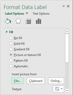
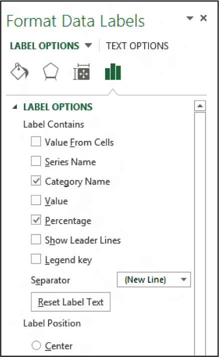
How to make a scatter plot in Excel - Ablebits Tick off the Data Labels box, click the little black arrow next to it, and then click More Options… On the Format Data Labels pane, switch to the Label Options tab (the last one), and configure your data labels in this way: Select the Value From Cells box, and then select the range from which you want to pull data labels (B2:B6 in our case). Excel data doesn't retain formatting in mail merge - Office In Excel, select the column that contains the ZIP Code/Postal Code field. On the Home tab, go to the Cells group. Then, select Format, and then select Format Cells. Select Number tab. Under Category, select Text, and then select OK. Save the data source. Then, continue with the mail merge operation in Word. References

Excel table styles and formatting: how to apply, change and remove On the Design tab, in the Table Styles group, click the More button. Underneath the table style templates, click Clear. Tip. To remove a table but keep data and formatting, go to the Design tab Tools group, and click Convert to Range. Or, right-click anywhere within the table, and select Table > Convert to Range.

Format data labels excel 2016

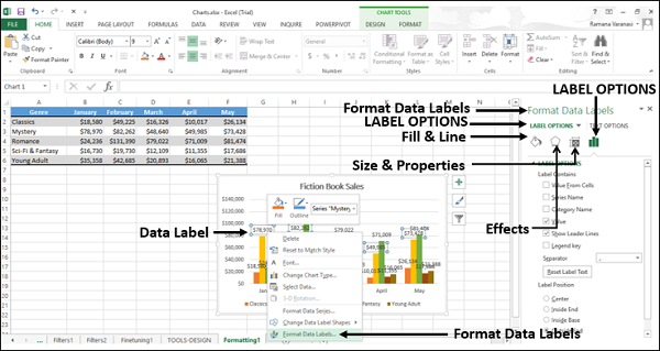
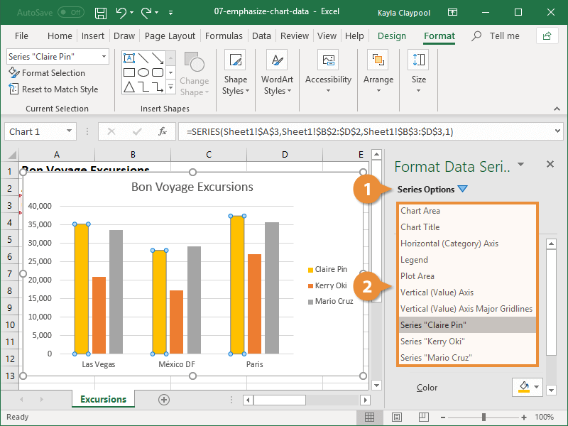
How to add secondary axis in Excel (2 easy ways) - ExcelDemy 2) Now right click on the Data Series and choose the Format Data Series option from the menu. 3) Format Data Series task pane appears on the right side of the worksheet. And we choose the Secondary Axis radio button for this data series. The keyboard shortcut to open this task pane is: CTRL + 1. Date format in Excel - Customize the display of your date To customize a date: Open the dialog box Custom Number (with the shortcut Ctrl + 1 or by clicking on the menu More number formats at the bottom of the number format dropdown) In this dialog box, you select ' Custom ' in the Category list and write the date format code in ' Type '. To format a date, you just write the parameter d, m or y a ... How to Add Labels to Scatterplot Points in Excel - Statology Step 3: Add Labels to Points Next, click anywhere on the chart until a green plus (+) sign appears in the top right corner. Then click Data Labels, then click More Options… In the Format Data Labels window that appears on the right of the screen, uncheck the box next to Y Value and check the box next to Value From Cells.

Format data labels excel 2016. Excel Conditional Formatting Data Bars On the Ribbon, click the Home tab, and then in the Styles group, click Conditional Formatting. In the list of conditional formatting options, click Data Bars, and then click one of the Data Bar options -- Gradient Fill or Solid Fill. (see tips below) The selected cells now show Data Bars, along with the original numbers. Excel Waterfall Chart: How to Create One That Doesn't Suck The first and last columns should be Total (start on the horizontal axis) and to set them as such, we have to double-click on each of them to open the Format Data Point task pane, and check the Set as total box. You can also right click the data point and select Set as Total from the list of menu options. Finally, we have our waterfall chart: 2. Data Labels bar chart - MrExcel I have extracted positive and negative values from column C to columns D and E using the simple formulas shown below the data. I selected B2:B7 then held Ctrl while also selecting D2:E7, and I inserted a clustered column chart (works with a bar chart also). I changed the overlap to 100%. (A stacked column chart has the overlap set to 100% by ... How to create a map chart - Get Digital Help Select data (A1:B56) Go to tab "Insert" on the ribbon Press with left mouse button on the "Maps" icon This world map shows up, US states are barely visible. This is not what we want. Back to top 3. Map Chart settings Double press with the left mouse button on the map to access chart formatting, see the image below.

Custom Excel number format - Ablebits To create a custom Excel format, open the workbook in which you want to apply and store your format, and follow these steps: Select a cell for which you want to create custom formatting, and press Ctrl+1 to open the Format Cells dialog. Under Category, select Custom. Type the format code in the Type box. Click OK to save the newly created format. Series.DataLabels method (Excel) | Microsoft Docs Example This example sets the data labels for series one on Chart1 to show their key, assuming that their values are visible when the example runs. VB Copy With Charts ("Chart1").SeriesCollection (1) .HasDataLabels = True With .DataLabels .ShowLegendKey = True .Type = xlValue End With End With Support and feedback Format Chart Axis in Excel - Axis Options However, In this blog, we will be working with Axis options, Tick marks, Labels, Number > Axis options> Axis options> Format Axis Pane. Axis Options: Axis Options There are multiple options So we will perform one by one. Changing Maximum and Minimum Bounds The first option is to adjust the maximum and minimum bounds for the axis. How to mail merge and print labels from Excel - Ablebits When the merge is finished, the placeholders will be replaced with the data from your Excel's address list. To arrange your address labels, follow these steps: In your Word document, click where you want to insert a field, and then click the corresponding link on the pane. For mailing labels, you'd normally need only the Address block.

Custom Chart Data Labels In Excel With Formulas Follow the steps below to create the custom data labels. Select the chart label you want to change. In the formula-bar hit = (equals), select the cell reference containing your chart label's data. In this case, the first label is in cell E2. Finally, repeat for all your chart laebls. Add data label using VBA and array - excelforum.com ActiveChart.FullSeriesCollection (1).DataLabels.Select ActiveChart.SeriesCollection (1).DataLabels.Format.TextFrame2.TextRange.InsertChartField msoChartFieldRange, "=TP01names", 0 ' TP01 is name array for data labels I tried to search for solution but unbale to understand the complexities and VBA code gives error. I am uploading the Xlsm file. How to Create a Run Chart in Excel (2021 Guide) | 2 Free Templates Go to the Insert tab. Click " Insert Line or Area Chart .". Choose " Line .". You now have your simple run chart as a result: Step 3. Spruce Up Your Run Chart. Technically, you're good to go, but if you're looking to improve your chart from boring to beautiful in mere moments, here's how you can quickly spruce it up. How to Create Labels in Word from an Excel Spreadsheet Select the Mailingstab at the top and then select Update Labels. All labels in your document should now say <>. 5. Create Labels From Excel in a Word Document Word now has all the data it needs to generate your labels. You will now finish the process and Word will display the actual data for each label:

Chart axes, legend, data labels, trendline in Excel - Tech Funda

DataLabels object (Excel) | Microsoft Docs The following example sets the number format for data labels on series one on chart sheet one. VB Copy With Charts (1).SeriesCollection (1) .HasDataLabels = True .DataLabels.NumberFormat = "##.##" End With Use DataLabels ( index ), where index is the data-label index number, to return a single DataLabel object.

Teach Besides Me: Data Labels Excel 2010

Chart.ApplyDataLabels method (Excel) | Microsoft Docs Syntax expression. ApplyDataLabels ( Type, LegendKey, AutoText, HasLeaderLines, ShowSeriesName, ShowCategoryName, ShowValue, ShowPercentage, ShowBubbleSize, Separator) expression A variable that represents a Chart object. Parameters Example This example applies category labels to series one on Chart1. VB Copy Charts ("Chart1").SeriesCollection (1).

How to Create a Chart in Microsoft Excel - TechSupport

How to: Create Excel 2016 Charts in the WinForms Spreadsheet Control Microsoft Excel 2016 introduced several chart types that help you visualize financial, statistical, and hierarchical data: Box and Whisker Waterfall Histogram Pareto Funnel Sunburst Treemap This topic describes how to use the Spreadsheet API to create and customize these chart types in your applications. Basics

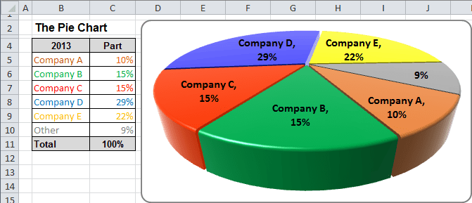
Excel 3-D Pie charts - Microsoft Excel 2010

Modifying Axis Scale Labels (Microsoft Excel) Follow these steps: Create your chart as you normally would. Double-click the axis you want to scale. You should see the Format Axis dialog box. (If double-clicking doesn't work, right-click the axis and choose Format Axis from the resulting Context menu.) Make sure the Number tab is displayed. (See Figure 1.) Figure 1.

Creating a simple competition chart - Microsoft Excel 2016

DataLabel object (Excel) | Microsoft Docs Use DataLabels ( index ), where index is the data-label index number, to return a single DataLabel object. The following example sets the number format for the fifth data label in series one in embedded chart one on worksheet one. VB Worksheets (1).ChartObjects (1).Chart _ .SeriesCollection (1).DataLabels (5).NumberFormat = "0.000"

Excel chart not printing correctly - i have a simple excel file (office

How to Print Labels from Excel - Lifewire Select Mailings > Write & Insert Fields > Update Labels . Once you have the Excel spreadsheet and the Word document set up, you can merge the information and print your labels. Click Finish & Merge in the Finish group on the Mailings tab. Click Edit Individual Documents to preview how your printed labels will appear. Select All > OK .

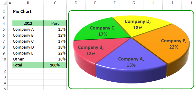
Excel 3-D Pie Charts - Microsoft Excel 2013

How to Create A Timeline Graph in Excel [Tutorial & Templates] On the top left, click Add Chart Element, then down to Data Labels followed by More Data Label Options. This opens the sidebar to format the data labels. Click Label Options and select Category Name under Label Contains. Change Label Position to Below. Now use the dropdown to select Series 1 (the hidden bar chart).

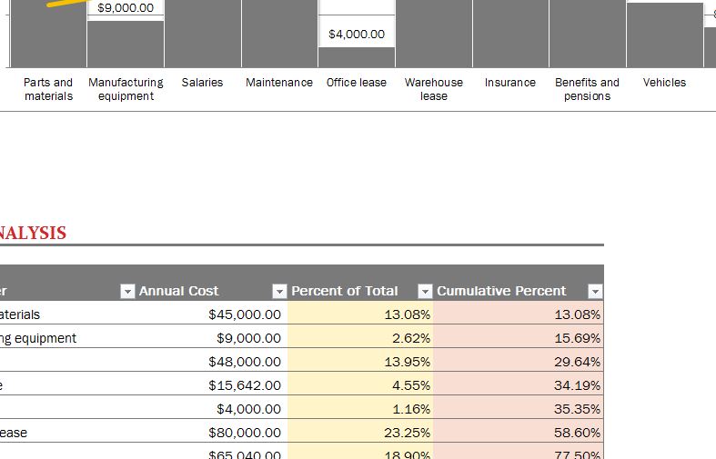
Cost Data & Chart Template - My Excel Templates

Two-Level Axis Labels (Microsoft Excel) - ExcelTips (ribbon) Make the cells at B1:G2 bold. (This sets them off from your data.) Place your row labels into column A, beginning at cell A3. Place your data into the table, beginning at cell B3. With your table completed, you are ready to create the chart. Just select your data table, including all the headings in the first two rows, then create your table.

Format Data Labels in Excel- Instructions - TeachUcomp, Inc.

How to Customize the Excel 2016 Ribbon with XML - dummies In the Custom UI Editor, choose File → Open and find the workbook you saved in Step 2. Choose Insert → Office 2007 Custom UI Part. Choose this command even if you're using Excel 2010, Excel 2013, or Excel 2016. Type the following code in the code panel (named customUI.xml) displayed in the Custom UI Editor:

Format Data Labels in Excel 2013- Tutorial - TeachUcomp, Inc.

How to Add Labels to Scatterplot Points in Excel - Statology Step 3: Add Labels to Points Next, click anywhere on the chart until a green plus (+) sign appears in the top right corner. Then click Data Labels, then click More Options… In the Format Data Labels window that appears on the right of the screen, uncheck the box next to Y Value and check the box next to Value From Cells.

Чарты Excel - Краткое руководство - CoderLessons.com

Date format in Excel - Customize the display of your date To customize a date: Open the dialog box Custom Number (with the shortcut Ctrl + 1 or by clicking on the menu More number formats at the bottom of the number format dropdown) In this dialog box, you select ' Custom ' in the Category list and write the date format code in ' Type '. To format a date, you just write the parameter d, m or y a ...